Student Mechanica: Research Paper

Showing posts with label Research Paper. Show all posts

Wednesday, 15 January 2014

Numerical Code: Prediction of Temperature distribution within Aluminium Alloy chip during orthogonal turning process

clear all
clc

% Eng. Ammar Aziz   Zohaib Hassan     Ahmad Bilal      Ali Hassan
%-------------------------------------------------------------------------
% Modeling of heat generation and Temperature distribution in machining
%-------------------------------------------------------------------------


%--------------------------------------------------------------------------
    %--------------------------------------------------------------
    % Heat generated in the Primary and Secondary deformation Zones
    %--------------------------------------------------------------

% The tool is standard C2 WC tool
% The chip is Al2024-T351.
hehe = input('Press any numeric key and then enter to start working=');

% Rake face angle of tool is

    alpha=input('rake face angle of tool(0 Radians is recommended for turning)=');
    rake_face_angle = num2str(alpha);
    display(rake_face_angle);

% Coefficient of friction between tool and chp
u = 0.57271;
coefficient_of_friction = num2str(u);
display(coefficient_of_friction);

% Normal friction angle in Radians
% Depends upon the coefficient of friction b/w tool and chip
    beta = atan(u);
    normal_friction_angle = num2str(beta);
    display(normal_friction_angle);

% Thickness of the cutted chip in meters is (found experimentally....)
t2 = 0.000333;
thickness_of_cutted_chip = num2str(t2);
display(thickness_of_cutted_chip);
% Contact length
cntct = 1.5*t2;

% Feed per revolution(in case of turning), in meters is given by
h = input('feed per revolution(0.000165 m/rev is standard)=');
feed_per_revolution = num2str(h);
display(feed_per_revolution);

% Chip thickness ratio is
    rat = h/t2;
    chip_thickness_ratio = num2str(rat);
    display(chip_thickness_ratio);

% Shear angle in the shear plane
% Depends upon the rake face angle and chip thickness ratio
    phi = atan((rat*cos(alpha))/(1-rat*sin(alpha)));
    shear_angle = num2str(phi);
    display(shear_angle);

% Width of the cutted chip in meters
w = 0.00254;
width_of_cutted_chip = num2str(w);
display(width_of_cutted_chip);

% Entering the shear strength of the chip283e6
S = 276e8;
shear_strength_of_chip = num2str(S);
display(shear_strength_of_chip);

% Cutting force in Newtons is given by (Merchant's circle approximation ..)
Fc = 573;
Cutting_Force = num2str(Fc);
display(Cutting_Force);

% Feed or Thrust force is Newtons is given by (Merchant's approximation..)
Ft = 329;
thrust_force = num2str(Ft);
display(thrust_force);

% Shear Force
Fs = Fc*cos(phi) - Ft*sin(phi);
shear_force = num2str(Fs);
display(shear_force);

% Shear area is given by
A_s = (h*w)/sin(phi);
shear_area = num2str(A_s);
display(shear_area);

% Shear stress within the primary zone is
tau = Fs/A_s;
shear_stress = num2str(tau);
display(shear_stress);

% The cutting velocity in meters per second is
Vw= 1.36;
cutting_velocity = num2str(Vw);
display(cutting_velocity);

% heat generation rate per unit depth of cut in primary zone :
Qs =(tau*h*Vw*cos(alpha))/(sin(phi)*cos(phi - alpha));
rate_of_heat_generation_in_primary_zone = num2str(Qs);
display(rate_of_heat_generation_in_primary_zone);
% heat generation rate for, length of cut as thickness of chip, in primary zone
Qso = Qs*t2;

% Frictional force acting between the rake face and chip is given by
Ff = Fc*sin(alpha) + Ft*cos(alpha);
frictional_force = num2str(Ff);
display(frictional_force);

% Rate of heat generation in the secondary zone is:
Qf =(tau*h*Vw*sin(beta))/(cos(phi + beta - alpha)*sin(phi - alpha));
rate_of_heat_generation_in_secondary_zone = num2str(Qf);
display(rate_of_heat_generation_in_secondary_zone);
% Rate of heat generation within contact length of secondary zone is:
Qfo = Qf*cntct;

%--------------------------------------------------------------------------

%--------------------------------------------------------------------------
                %------------------------------------
                %Average temperature rise calculation
                %------------------------------------
% Thermal conductivity of the workpiece in watts per meter per kelvin
Kc=177;

% Mass density of chip in kilograms per cubic meter
p=2785;

% specific heat capacity of chip in joules per kilogram per kelvin
Cc=875;

% Thermal Diffusivity
Sa = Kc/(p*Cc);

% Thermal number
Rt = (h*Vw)/Sa;

% fraction of heat flowing into the tool
X = 0.5 - (0.35* (log10(Rt*tan(phi))));

% Average temperature rise of the (((chip))) per unit depth of cut due to shearing
delta_T = ((1-X)*Qs)/(p*Cc*h*Vw);
average_temp_rise = num2str(delta_T);
display(average_temp_rise);
%This average temperature rise on the shear plane is used as a boundary
%condition at the upper left corner of the chip

%-------------------------------------------------------------------------


%--------------------------------------------------------------------------
                    %------------------
                    %Mesh generation
                    %------------------

% Chip velocity, for unit depth of cut, is given as
Vc = Qf/Ff;
chip_velocity = num2str(Vc);
display(chip_velocity);

% No of grids in x-direction
nbx = input('please enter no. of grids in x-direction (4 is default)=');
%No of grids in y-direction
nby = input('please enter no. of grids in y-direction (4 is default)=');

% No of nodes in x-direction
nbnx = nbx + 1;
% No of nodes in y-direction
nbny = nby + 1;

% proportion of frictional heat entering into the tool
Tio = 0.03;

% Grid spacing in x-direction
grsx = cntct/nbx;

% Grid spacing in y-direction
grsy = t2/nby;

% No. of nodes in the mesh
nod = nbnx*nbny;

% heat flow rate in chip's primary control zone due to primary zone heat source is
Qrs = ((1-Tio)*Qs*grsy)/t2;
heat_flow_in_chip_node_due_to_shear_source=num2str(Qrs);
display(heat_flow_in_chip_node_due_to_shear_source);

% heat generation rate for a secondary node in chip due to frictional heat source
Qrf = ((1 - Tio)*Qf*grsx)/cntct;
heat_flow_in_chip_due_to_frictional_source=num2str(Qrf);
display(heat_flow_in_chip_due_to_frictional_source);

% Heat generation array
hga = [];
for i= 1:((sqrt(nod)));
hga(i,sqrt(nod)) = Qrf;
end

for j= 1:((sqrt(nod))-1)
    for k = 1:(sqrt(nod)-1)
    hga(k,j) = 0;
    end
end

for m=1:(sqrt(nod)-1)
hga(sqrt(nod),m) = Qrs;
end

hga(sqrt(nod),sqrt(nod)) = Qrf + Qrs;
display(hga);

%temperature distribution within the chip

Am0 = (p*Cc*Vc)/(Kc);
Am1 = Am0/grsx;
Am2 = - (2/(grsx^2)) - (2/(grsy^2)) + Am1;
Am3 = (1/(grsx^2)) - (Am1);
Am4 = (grsx^2)*(grsy^2);
Am5 = Am4 * Am2;
Am6 = Am4 * Am3;
Am7 = grsy^2;
Am8 = grsx^2;
Am9 = Qrf/Kc;
A_1 = Am6/Am5;
A_2 = Am7/Am5;
A_3 = Am8/Am5;
A_4 = Am9/Am5;
A1 = -A_1;
A2 = -A_2;
A3 = -A_3;
A4 = -A_4;

for M = 1: (nbx - 1)
xM = M*grsx;
end

for N = 1: (nby - 1)
xN = N*grsy;
end

tempi = [];

% Boundary Condition
tempi(sqrt(nod),1) = delta_T;

% Data is imported from Solidworks 2012 by applying the boundary conditions
tempi = [344.1 345 346.1 347.3 350.3; 343 344.2 345.4 347.8 350.3; 339 336.9 343.9 348 351.2; 329.9 335.6 341.3 354.4 356.1; 234.5 343.1 352.7 362.4 370.6];
display(tempi);

% matrix of coefficients is given by
coeffik = (inv(tempi))*hga;
display(coeffik);

% Temperature distribution within the chip is given by multiplying inverse
% of coefficient matrix with heat generation array.

% plotting temperature
[x,y]=meshgrid(1:sqrt(nod),1:sqrt(nod));
surf(x,y,tempi)

%--------------------------------------------------------------------------
%THE END
%--------------------------------------------------------------------------
%--------------------------------------------------------------------------

Prediction of Temperature distribution within Aluminium Alloy chip during orthogonal turning process

By: Engr. Ammar Aziz, Engr. Zohaib Hassan, Engr. Ahmad Bilal, Engr. Ali Hassan
COMSATS University of Science and Technology Sahiwal, Pakistan

Abstract
In this paper, a numerical model based on finite difference method is presented to predict chip temperature field in orthogonal turning process. Orthogonal turning can be studied by modeling the heat transfer between tool and chip at tool-rake face contact zone. The mathematical model and simulation results, presented here, are in satisfactory agreement with experimental temperature measurement reported in the literature.

1- Preparing Numerical Model
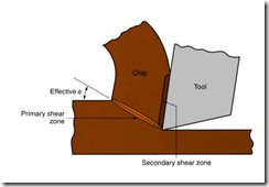
First of all consider the orthogonal turning process. Heat is generated within the chip due to its interaction with the tool. This heat generation is sub-divided into primary heat generation zone and secondary heat generation zone, as shown in the following figure:

Here ‘phi’ is the shear angle. It is the angle of the shear plane with the horizontal axis.

Rate of heat generation, per unit depth of cut within primary shear zone is given by:

Rate of heat generation within secondary shear zone is given by:

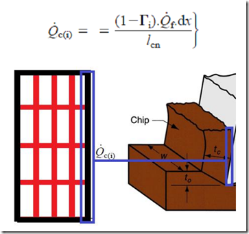
Average temperature rise of chip per unit depth of cut due to shearing:

This temperature rise is used as a boundary condition at the point shown in the figure:

Finite Difference Method and Derivative Concept:
Before proceeding to further modification, it is first necessary to clear that what is the meaning of a derivative and why we are relating it with finite difference concept. Also what does mean by partial derivative?

Meshing of our chip with 25 nodes

First law of thermodynamics implementation
Supposing a control zone within the mesh and applying the law of conservation of energy there we get:

According to Fourier’s law of heat conduction:

Substituting the values from Fourier’s law into heat balance equation we get:

Now by using the concept of Taylor series expansion about a point….

Approximating partial derivatives using forward and backward difference simultaneously, we get:

So our final model is ……

Heat flow in differential chip control zone from the frictional heat source is:

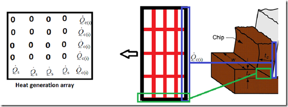
So heat generation array can be constructed by putting the value from above formula into all entries of last column and putting the value of heat generated in primary zone, in last row. All the entries except which described above are zero because here there is no heat generation as shown in the following figure:

At last we determine the coefficients matrix which is obtained by solving the final model equation for each node of the chip and determining the coefficients through algebraic manipulations.

The purpose of above picture is to show you something interesting. As we write
the equation for each node the coefficients jump to next variable by one step. So if we try to write the above equations in matrix form than the matrix of
coefficients contain the entries which move diagonally. Siedal algorithm is best
to write the matrix of this type. The inverse of coefficient matrix is when multiplied by the heat generation array then we get the temperature distribution array which is our goal.

Plot of temperature against the distances along the edges of the chip in MATLAB:

Contour Plot:

Simulation of chip:
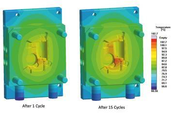
Solid works 2012 is used to accomplish the simulation of chip.

Description
Prediction of temperature distribution within chip of Aluminium. The tool which is used for turning process is made up of ‘C2 WC’.

Meshing…………..

Comment: The results are very close to those which are practically observed

Tuesday, 14 January 2014

Trajectory Research about the Rolling-Pin Belt Transmission

Abstract: A new belt transmission mechanism, having the function of no-slip driving, is described in the paper. It is composed of pulleys with carved rails and belt with rolled pins spaced out on both sides. Firstly, the trajectory curve is deduced along which pins embedded in the pulley. And then, parametric relationships are established, which are about center offsets of two pulleys, working radius of each pulley, the number of meshing curves on every pulley and the number of pins on the belt. All of those provide a theoretical basis for the design of this type of no-slip belt transmission mechanisms.

Work Download the manual now

Finite volume method for simulating extreme ﬂood events in natural channel

he need for mitigating damages produced by extreme hydrologic events has stimulated the European Community to fund several projects. The Concerted Action on Dam-break Modelling workgroup (CADAM) performed a considerable work for the development of new codes and for the adequate veriﬁcation of their performance. In the context of the CADAM project, a new 2D computer code is developed, tested and applied, as described in the present paper. The algorithm is obtained through the spatial discretisation of the shallow water equations by a ﬁnite volume method, based on the Godunov approach. The HLL Riemann solver is used. A second order accuracy in space and time is achieved, respectively by MUSCL and predictor–corrector techniques. The high resolution requirement is ensured by satisfaction of TVD property. Particular attention is posed to the numerical treatment of source terms. Accuracy, stability and the reliability of the code are tested on a selected set of study cases. A grid reﬁnement analysis is performed. Numerical results are compared with experimental data, obtained by the physical modelling of a submersion wave on a portion of the Toce river valley, Italy, performed by ENEL–HYDRO and considered as representative of a real life ﬂood occurrence.

Work Download paper now

Numerical study of simultaneous natural convection heat transfer from both surfaces of a uniformly heated thin plate

Abstract Numerical studies were conducted to investigate the natural convection heat transfer around a uniformly heated thin plate with arbitrary inclination in an infinite space. The numerical approach was based on the finite volume technique with a no staggered grid arrangement.For handling the pressure±velocity coupling the SIMPLE-algorithm was used. QUICK scheme and ®rst order up-wind scheme were employed for discretization of the momentum and energy convective terms respectively. Plate width and heating rate were used to vary the modified Rayleigh number over the range of 4:8 Â 10 6 to 1:87 Â 10 8. Local and average heat transfer characteristics were compared with regarding to the inclination angle.The empirical expressions for local and average Nusselt number were correlated. It has been found that for incli-nation angle less than 10, the ¯ow and heat transfer characteristics are complicated and the average Nusselt number can not be correlated by one equation while for inclination angle larger than 10, the average Nusselt number can be correlated into an elegant correlation.

Work Download Paper Now

Modeling Dynamic Rupture in 3D earthquake fault model

An earthquake (also known as a quake, tremor or temblor) is the result of a sudden release of energy in the Earth's crust that creates seismic waves. The seismicity, seismism or seismic activity of an area refers to the frequency, type and size of earthquakes experienced over a period of time.

Earthquakes are measured using observations from seismometers. The moment magnitude is the most common scale on which earthquakes larger than approximately 5 are reported for the entire globe. The more numerous earthquakes smaller than magnitude 5 reported by national seismological observatories are measured mostly on the local magnitude scale, also referred to as the Richter scale. These two scales are numerically similar over their range of validity. Magnitude 3 or lower earthquakes are mostly almost imperceptible or weak and magnitude 7 and over potentially cause serious damage over larger areas, depending on their depth. The largest earthquakes in historic times have been of magnitude slightly over 9, although there is no limit to the possible magnitude. The most recent large earthquake of magnitude 9.0 or larger was a 9.0 magnitude earthquake in Japan in 2011 (as of October 2012), and it was the largest Japanese earthquake since records began. Intensity of shaking is measured on the modified Mercalli scale. The shallower an earthquake, the more damage to structures it causes, all else being equal.^[1]

At the Earth's surface, earthquakes manifest themselves by shaking and sometimes displacement of the ground. When the epicenter of a large earthquake is located offshore, the seabed may be displaced sufficiently to cause a tsunami. Earthquakes can also trigger landslides, and occasionally volcanic activity.

In its most general sense, the word earthquake is used to describe any seismic event — whether natural or caused by humans — that generates seismic waves. Earthquakes are caused mostly by rupture of geological faults, but also by other events such as volcanic activity, landslides, mine blasts, and nuclear tests. An earthquake's point of initial rupture is called its focus or hypocenter. The epicenter is the point at ground level directly above the hypocenter.

Work Download paper now

Use of Computational Fluid Dynamics to Predict Airflow and Contamination Concentration Profiles Within Laboratory Floor Plan Environment

Eliminating environmental or other airborne contaminants in medical, biological research and production facilities is critical to the success of their mission (Sansone & Losikoff, 1977; Walters & Ryan, 2001). In situ measurement of environmental conditions creates a potential for inhalation hazards. Use of computational fluid dynamics (CFD), allows for a non-intrusive way of determining the room air conditions without concern for operator safety. The goal of this study is to use CFD computer modeling to study a pharmaceutical clean-room environment in which there has been an accidental introduction of aerosolized contaminant. The concentration and distribution of the contaminant is determined throughout the room for a range of conditions, by computation using three mathematical models and also experimentally field deter-mined. A comparison of best fit shows High Reynolds number k-İ model calculations are most practical from a computational and prediction standpoint.